S-scenario
Map parameters
S-scenario considers a model of a town in 🇦🇹. Specifically, the region of interest (ROI) is the town of Schwechat (near Vienna) and the railway track of the main 🚆 operator in 🇦🇹, ÖBB.
Map parameters
ROI OSM coordinate system WGS-84:
- Max. latitude = 48.1505
- Min. latitude = 48.1439
- Min. longitude = 16.4633
- Max. longitude = 16.4778
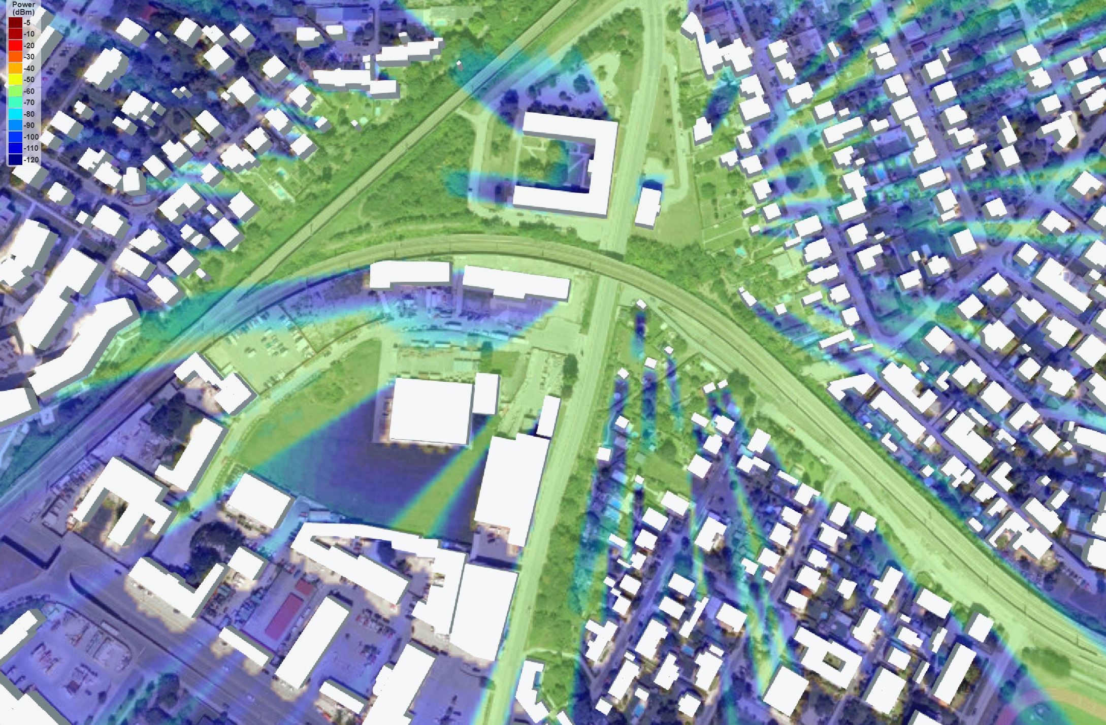
The dataset is based on the map shown below for $r$-th transmitter location $\mathbf{u} _{r}$ and a single BS at $\mathbf{b} _{m}$.

3D models
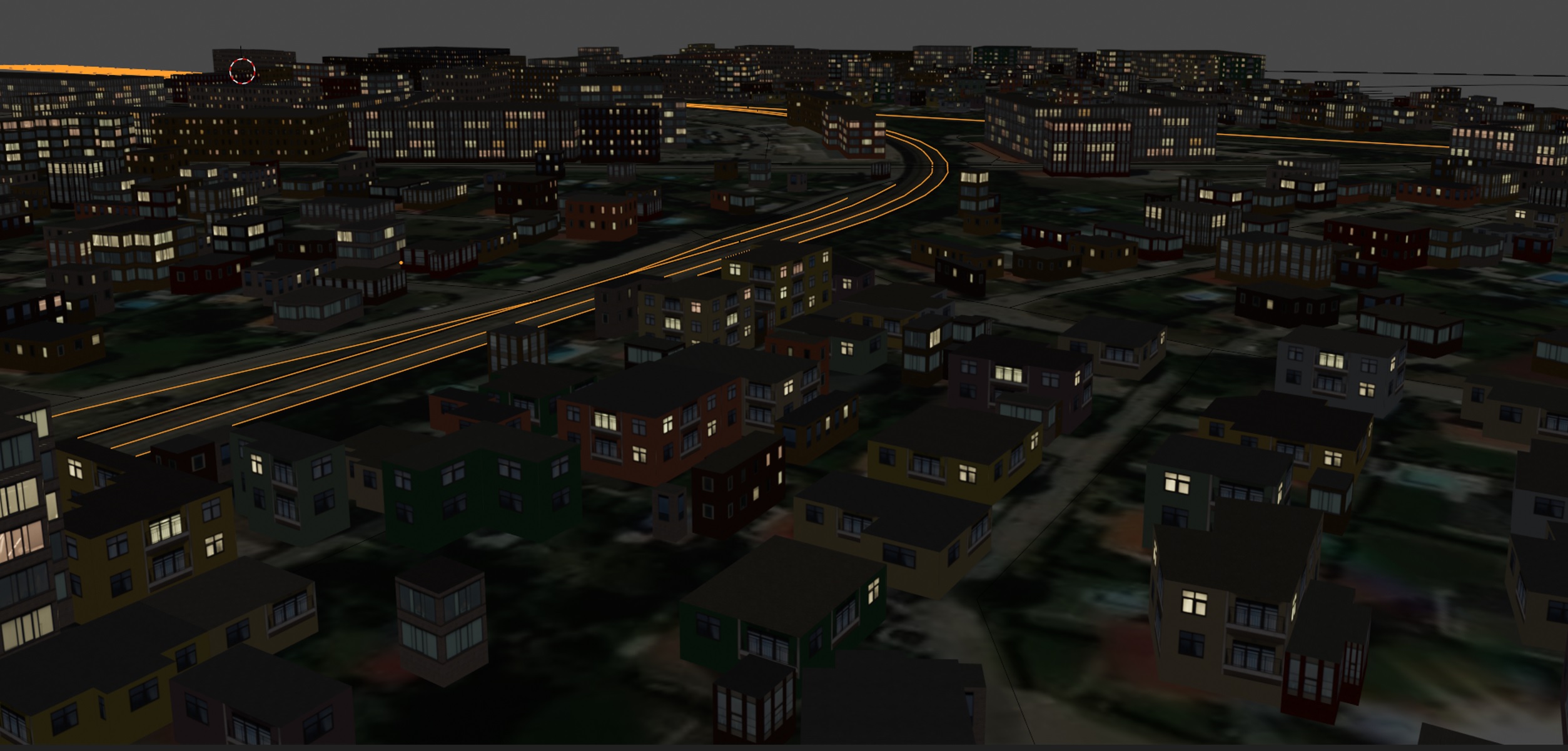
Below, is an example of the 3D model of S-scenario. In addition to buildings and available objects from the OSM, this scenario contains other objects, such as cars and a train passing by that do change their position for every time-snapshot.
Scenario parameters
S-scenario 3D models:
- $T$ = 200.
- 1 train
- $\approx 70$m long
- $\approx 4$m height
- $\approx 3.25$m width
- 4 cars.
- $\approx 4.70$m long
- $\approx 1.8$m height
- $\approx 1.9$m width

3D models are provided in STL or SKP format. STLs can be opened by any CAD tool, while SKPs are specific to SketchUp. State of the art wireless ray-tracing tools should support this format. STL files can be downloaded from our owncloud. Similarly, you can download SKP files from owncload.
Download the dataset - STL Models.
Scenario files here are all in .stl format. The dataset is compressed into a .zip file. Depending the scenario and the details of the environment, a size of each file can be 1 up to 5 MB.
Download the dataset - SKP Models.
Scenario files are all in .skp format. The dataset is compressed into a .zip file. Depending the scenario and the details of the environment, a size of each file can be 1 up to 5 MB.
Ray-traces (RT)
All path parameters values between the BS and user location are obtained using the ray-tracer available in Matlab®. The dataset contains traces for $T=200$ and a single-BS.
RT parameters
S-scenario ray traces:
- SBR ray-tracing approach.
- Low-angular resolution with $\approx 655,362$ rays.
- Receiver sensitivity $\geq \text{-}130\text{dBm}$.
- $T$ = 200.
- $R$ = 360.
- $b_{m,3} = 20 \textrm{ m}$.
- $u_{m,3} = 1.5 \textrm{ m}$.
- $f _{c} = 3.5 \textrm{ GHz}$.
- EM properties of the scattering objects change over the time
- $\kappa \in{\text {concrete, brick, metal, wood}}$.
- Rainy periods $\mathcal{R}$ with $\mathbb{P}(\mathcal{R}) = 1/3.$
All obtained ray traces are provided in .mat file format and can be opened using Matlab or Python. The files can be from our owncloud.
Download the dataset
There is only one RT file in .mat format. There $69\,212$ samples. The size of the structure is relatively low, thus can be easily fit to memory of any modern computer. The total size is $\approx72\textrm{MB}$. Download the dataset in a compressed .zip file.
Channel state information (CSI)
To obtain the channel from the RT, we consider a geometric channel model. CSI is stored as $\mathbf{H} _{r}^{t} =\left[\mathbf{\widehat{h}} _{k _1}^{t}, \mathbf{\widehat{h}} _{k _2}^{t}, \ldots, \mathbf{\widehat{h}} _{k _{N _{c}’}}^{t}\right] \in \mathbb{C}^{N _{r} \times N _{c}’} .$ Dataset has channel and location pairs.
CSI parameters
S-scenario CSI:
- $M = 1$.
- $N_{c} = 512$, $N_{c}’ = 32$ and $N_{c} \equiv N_{c}’ \quad(\bmod ; 16)$.
- $L = 4$.
- $B = 20 \textrm{ MHz}$.
- Estimation subcarriers
- $\widehat{\mathbf{h}} _{k}^{t} = \sum _{\ell=1}^{L} \eta _{\ell}^{t} e^{j{2 \pi k}{\Delta f} \tau _{\ell}^{t}} \mathbf{a}\left(\varphi _{a z,\ell}^{t}, \varphi _{e l,\ell}^{t} \right) . $
Obtained CSI are provided in .mat file format and can be opened using Matlab or Python. The files can be from our owncloud.
Download the dataset
There is only one CSI file in .mat format. The size of the structure is relatively low, thus can be easily fit to memory of any modern computer. The total size is $\approx 2.31 \textrm{GB}$. Download the dataset in a compressed .zip file.
BJTU Datasets

BJTU Ray-tracer
The BJTU ray-tracer is available at http://cn.raytracer.cloud:9090/. The ray-tracer is developed by the Beijing Jiaotong University.
Path parameters are also obtained via BJTU-RT. The S-200 dataset now is obtained in 30 GHz frequency band.
RT parameters
S-scenario ray traces:
- $T$ = 200.
- $R$ = 349.
- $b_{m,3} = 25 \textrm{ m}$.
- $u_{m,3} = 1.5 \textrm{ m}$.
- $f _{c} = 30.00 \textrm{ GHz}$.
All obtained ray traces are provided in .mat file format and can be opened using Matlab or Python. Due to very large size of the dataset, please contact us and we will provide you with the dataset.
Download the dataset
There are multiple files in .mat format, saved under ''' ./results/
Download the dataset in mmWaves
Download the channels for the dataset in 30 GHz (CTF from BJTU-RT).
Download the dataset in mmWaves
Download the labels for the dataset in 30 GHz (CTF from BJTU RT).
Showcase
As the 5G mobile services start penetrating worldwide, in many B5G / 6G visions disclosed, we can find Digital-Twins, Society 5.0, etc., where wireless technologies take one significant role as the social infrastructure.
We believe that simulating the real-life conditions will be crucial for the future of wireless technologies to understand how the surrounding dynamics impact the 5G and beyond systems. A real-time virtual city-scale digital twins will be a new norm for analyzing and designing future mobile communications systems.
In addition to scientific methododology for evaluating the performance, we transfer the knowledge to more realistic environment to showcase our work for the industry partners.
MPC visualization
An example of the communication of a transmitter along the railway track is shown below. We are looking at the PDP of the transmitter along the track. Moreover, we can observe the expected driving route and estimated locations.
When our DNN is not sure of a prediciton, it associates a high uncertainty to its estimate. Check the in action starting at 00:23.
- MPCs
- Actual map
- PDP profile
- Location estimates
- Uncertainty estimates
Mobility and time-varying environment
The dataset with all 3D models is a time-varying environment. Buildings, cars, and other object change their position every time snapshot. A train moves parallel to the track considered for the transmitter. Another object moving parallel to the train is introduced to stretch the impact of multipath components.